Random Variable Normal Distribution Comparisons Agains Other Event

Learning Outcomes

• Employ a normal probability distribution to gauge probabilities and identify unusual events.

Now we utilise the simulation and the standard normal curve to find the probabilities associated with any normal density curve.

Example

Length of Man Pregnancy

The length (in days) of a randomly called human pregnancy is a normal random variable with μ = 266, σ = xvi. So X = length of pregnancy (in days)

(a) What is the probability that a randomly chosen pregnancy will last less than 246 days?

We desire P(Ten < 246). To detect this probability, we outset catechumen Ten = 246 to a z-score:

[latex]Z=\frac{246-266}{16}=\frac{-twenty}{16}=-one.25[/latex]

Now we tin can employ the simulation to detect P(Z < −i.25). This is the surface area under the normal probability curve to the left of Z = −1.25.

The probability that a randomly chosen pregnancy lasts less than 246 days is 0.1056. In other words, there is an 11% chance that a randomly selected pregnancy volition last less than 246 days.

(b) Suppose a significant woman's husband has scheduled his business trips then that he will be in town between the 235th and 295th days of her pregnancy. What is the probability that the birth volition have place during that time?

Compute the z-scores for each of these 10-values:

[latex]Z=\frac{235-266}{16}=\frac{-31}{16}=-ane.94[/latex]

and

[latex]Z=\frac{295-266}{xvi}=\frac{29}{16}=1.81[/latex]

Apply the simulation to find the area nether the standard normal curve betwixt these ii z-scores.

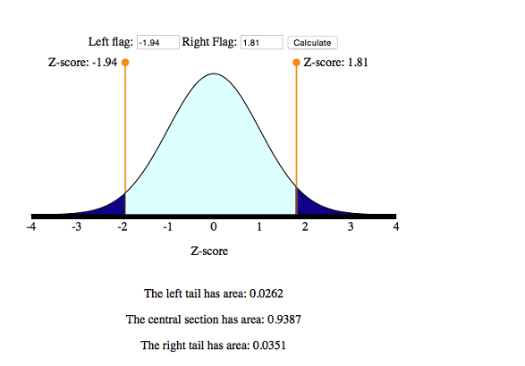
So the desired probability is 0.9387.

[latex]P(235<10<295)=P(-ane.94<Z<ane.81)=0.9387[/latex]

There is about a 94% probability that he will be home for the nativity. Looks like he planned well.

Endeavour It

The previous examples all followed the same general form: Given values of a normal random variable, nosotros found an associated probability. The two basic steps in the solution process were as follows:

1. Convert x-value to a z-score.
2. Utilise the simulation to find associated probability.

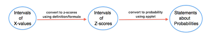
The side by side example is a different type of trouble: Given a probability, we volition observe the associated value of the normal random variable. The solution process volition get in reverse order.

1. Use a new simulation to convert statements about probabilities to statements virtually z-scores.
2. Catechumen z-scores to ten-values.

These types of problems are informally called "work-backwards" issues. We will apply a new simulation for these types of problems. The new simulation requires us to enter a probability and so gives usa the associated z-score. This is backwards from the simulation we worked with previously where nosotros entered a z-score to find a probability. Nosotros will use this simulation in the side by side example.

Click hither to open up this simulation in its own window.

Example

Work Backwards to Find Ten

Foot length (in inches) of a randomly chosen adult male is a normal random variable with a mean of 11 and standard deviation of 1.five. And so X = pes length (inches).

(a) Suppose that an XL sock is designed to fit the largest 30% of men's feet. What is the smallest foot length that fits an XL sock?

Pace 1: Utilise the simulation to catechumen the probability to a statement virtually z-scores.

Nosotros want to mark off the largest 30% of the distribution, so the probability to the correct of the z-score is 30%. This means that lxx% of the surface area is to the left of the z-score.

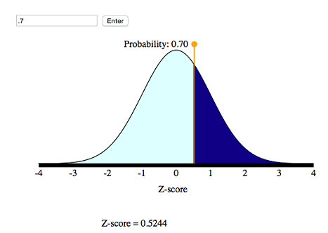
From the simulation, nosotros tin come across that the corresponding z-score is 0.52.

Step 2: At present we need to convert this z-score to a foot length.

Before we calculate the length, note that the z-score is about 0.5, so the x-value will exist about 0.5 standard deviations higher up the mean.

[latex]10=\mathrm{μ}+0.5⋅\mathrm{σ}=11+0.5(i.5)=11+0.75=11.75\text{}\mathrm{inches}[/latex]

Conclusion: A human foot length of 11.75 inches is the shortest human foot for an Twoscore sock.

(b) What is the first quartile for the men'south pes lengths?

Pace 1: Use the simulation to catechumen this probability into a statement about z-scores.

We want to marker off the smallest 25% of the distribution, and then the probability to the left of the z-score is 25%.

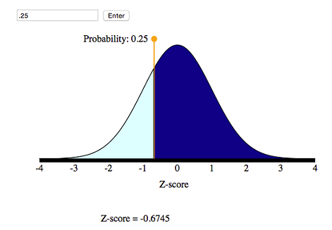
From the simulation, we can see that the corresponding z-score is −0.67.

Pace two: Convert this z-score to a pes length. If 10 is the foot length nosotros seek, then X is 0.67 standard deviations below the mean. That is,

[latex]ten=\mathrm{μ}-0.67⋅\mathrm{σ}=eleven-0.67(i.5)=11-one.005=9.995\text{}\mathrm{inches}[/latex]

Determination: The start quartile mark is 9.995 inches, so about 25% of the men'south anxiety are shorter than ten inches.

Comments

In the preceding example (specifically stride 2), nosotros found the x-value by reasoning about the meaning of the z-score. We can also develop a formula for this procedure.

Recall the definition of z-score. In words, the z-score of an x-value is the number of standard deviations X is away from the mean. As a formula, this is

[latex]Z=\frac{ten-\mathrm{μ}}{\mathrm{σ}}[/latex]

We tin solve this equation for 10 equally follows:

[latex]\brainstorm{assortment}{l}\frac{ten-\mathrm{μ}}{\mathrm{σ}}=Z\\ 10-\mathrm{μ}=Z⋅\mathrm{σ}\\ 10=\mathrm{μ}+Z⋅\mathrm{σ}\cease{array}[/latex]

This gives united states a formula for finding X from Z. You lot can use this formula in footstep 2 of a work-backwards problem.

Endeavour It

Let'southward Summarize

• In "Continuous Random Variables," we made the transition from detached to continuous random variables. A continuous random variable is non limited to distinct values. It is a measurement such as human foot length. We cannot display the probability distribution for a continuous random variable with a table or histogram. We apply a density bend to assign probabilities to intervals of 10-values. We use the area under the density curve to find probabilities.
• We use a normal density curve to model the probability distribution for many variables, such as weight, shoe sizes, foot lengths, and other human being concrete characteristics. Normal curves are mathematical models. We use µ to correspond the hateful of a normal bend and σ to represent the standard deviation of a normal bend. We utilise Greek letters to remind us that the normal bend is non a distribution of real information. It is a mathematical model based on a mathematical equation. Nosotros employ this mathematical model to correspond the perfect bong-shaped distribution.
• For a normal curve, the empirical rule for normal curves tells us that 68% of the observations autumn within 1 standard departure of the mean, 95% within two standard deviations of the mean, and 99.vii% within three standard deviations of the mean.
• To compare x-values from different distributions, we standardize the values by finding a z-score:[latex]Z=\frac{x-\mathrm{μ}}{\mathrm{σ}}[/latex]
• A z-score measures how far X is from the mean in standard deviations. In other words, the z-score is the number of standard deviations X is from the mean of the distribution. For case, Z = i means the x-value is 1 standard difference to a higher place the mean.
• If we convert the x-values into z-scores, the distribution of z-scores is as well a normal density curve. This curve is called the standard normal distribution. We utilise a simulation with the standard normal bend to observe probabilities for any normal distribution.
• We tin can also piece of work backwards and notice the ten-value for a given probability. We used a different simulation to work backwards from probabilities to x-values. With this simulation, we found x-values respective to quartiles and percentiles.

Are You Set up for the Checkpoint?

If you completed all of the exercises in this module, you should be fix for the Checkpoint. To make sure that you are ready for the Checkpoint, apply the My Response link below to evaluate your understanding of the learning outcomes for this module and to submit questions that yous may take.

davidpriarriank02.blogspot.com

Source: https://courses.lumenlearning.com/wmopen-concepts-statistics/chapter/introduction-to-normal-random-variables-6-of-6/

Share this post